Death and Minimum Legal Drinking Age in the US

In a regression discontinuity design, we compare people who are just above some cutoff with those who are just below, where the treatment is determined by the cutoff. The essential idea is conveyed by the following dialogue between Master Stevefu and the Grasshopper in Angrist and Pischke’s (2015, p.175) book Mastering Metrics:

MASTER STEVEFU: Summarize RD for me, Grasshopper.

GRASSHOPPER: The RD design exploits abrupt changes in treatment status that arise when treatment is determined by a cutoff.

MASTER STEVEFU: Is RD as good as a randomized trial?

GRASSHOPPER: RD requires us to know the relationship between the running variables and potential outcomes in the absence of treatment. …

MASTER STEVEFU: How can you know that your control strategy is adequate?

GRASSHOPPER: One can’t be sure, Master. But our confidence in causal conclusions increases when RD estimates remain similar as we change details of the RD model.

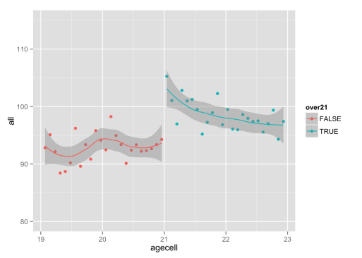
My friend Kanishka Kacker first told me about the particular importance of graphs in regression discontinuity designs. In their fine review of regression discontinuity, Lee and Lemieux (2010) write: “It has become standard to summarize RD analyses with a simple graph showing the relationship between the outcome and assignment variables. This has several advantages. The presentation of the ‘raw data’ enhances the transparency of the research design. A graph can also give the reader a sense of whether the ‘jump’ in the outcome variable at the cutoff is unusually large compared to the bumps in the regression curve away from the cutoff. … The problem with graphical presentations, however, is that there is some room for the researcher to construct graphs making it seem as though there are effects when there are none, or hiding effects that truly exist.”

In this example taken from Mastering Metrics, the minimum legal drinking age can affect drinking and thereby such behaviour as drinking under the influence of alcohol. We can study the effect of legal access to alcohol on death rates.

We read in the data (relating to Chapter 4), available on the Mastering Metrics website (http://masteringmetrics.com/resources/).

library(foreign)
mlda=read.dta("AEJfigs.dta")

We then create a dummy for age over 21.

mlda$over21 = mlda$agecell>=21
attach(mlda)

We then fit two models, the second has a quadratic age term.

fit=lm(all~agecell+over21)
fit2=lm(all~agecell+I(agecell^2)+over21)

We plot the two models fit and fit2, using predicted values.

predfit = predict(fit, mlda)
predfit2=predict(fit2,mlda)
# plotting fit
plot(predfit~agecell,type="l",ylim=range(85,110),
     col="red",lwd=2, xlab="Age",
     ylab= "Death rate from all causes (per 100,000)")
# adding fit2
points(predfit2~agecell,type="l",col="blue")
# adding the data points
points(all~agecell)

Death rates from all causes against age . Red line is model fit and blue line is model fit2.

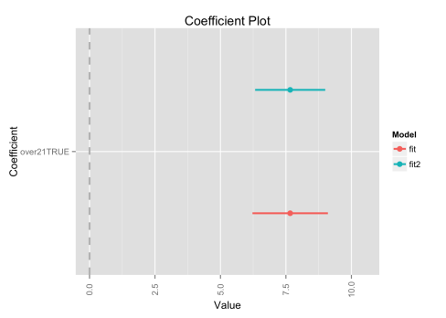
We can plot the confidence intervals for the coefficients in the two models; they are very similar.

library(coefplot)
multiplot(fit,fit2,predictors="over21")

Confidence intervals plot for variable over21 in the models fit and fit2.

We can also plot the data and use a loess smoother for age below and above 21.

library(ggplot2)
age3=ggplot(mlda, aes(x = agecell, y = all,colour=over21)) + 
  geom_point() + ylim(80,115)
age4=age3 + stat_smooth(method = loess)
age4

R has a specialized package called “rdd” for regression discontinuity analysis. We won’t pursue it here.

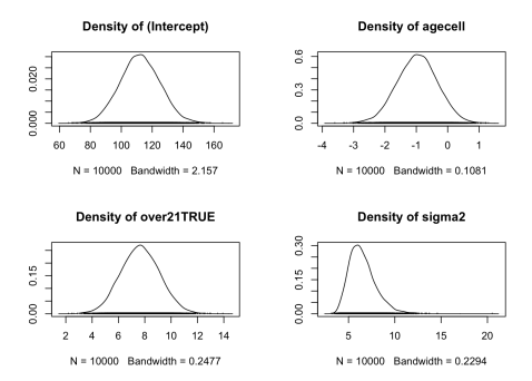
We can do a quick Bayesian analysis in R with the MCMCpack package.

library(MCMCpack)
pos=MCMCregress(all~agecell+over21, data=mlda,verbose=FALSE)
plot(pos,trace = FALSE)

Our quantity of interest is over21TRUE.

References

Angrist J D, Pischke J-S (2015). Mastering Metrics: The Path from Cause to Effect. Princeton University Press.

Lee D S, Lemeiux T (2010) Regression Discontinuity Designs in Economics. Journal of Economic Literature (June 2010): 281-355